ANNA'S ANALYTICS

Bayes' Bulls

Okay so I am definietly not a cowgirl, but as soon as summer hits, I start dreaming about driving with the windows down, blasting country music. I’ve been to a few rodeos and always have a great time, but I know nothing about rodeo sports. I came across some bull riding data on GitHub and thought, “Why not?” So here’s me, learning how bull riding actually works and doing a quick Bayesian analysis.

Bull Riding 101

For those of you who are like me and know nothing about bull riding, here’s the gist of the sport and the scoring:

Data

I got my data from the 2023 Unlease the Beast league which is the highest level of professional bull riding. One thing that stood out to me was that the top rider in 2023, Rafael José de Brito, had some of the lowest metrics among the top competitors.

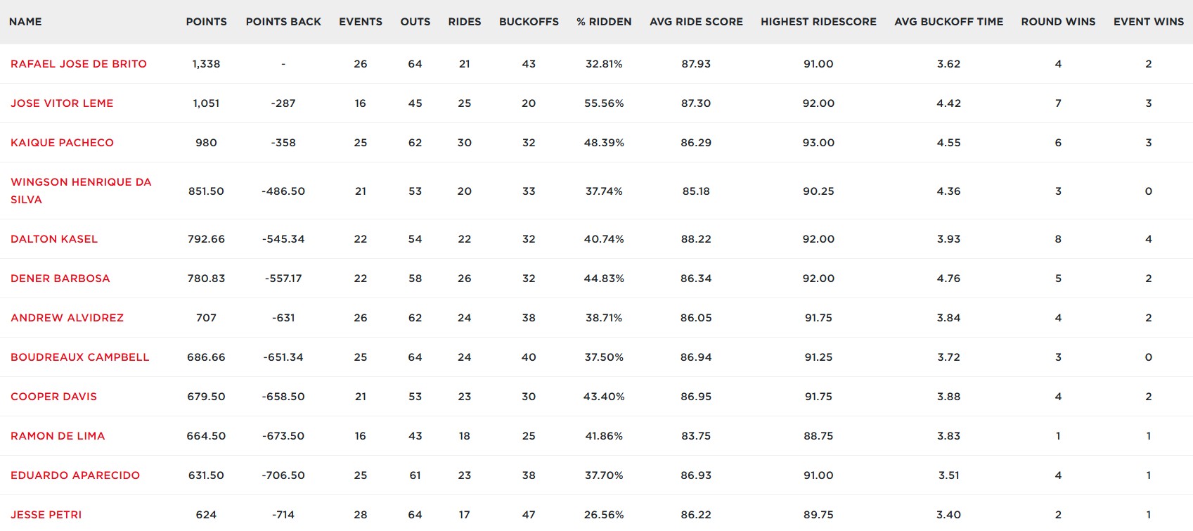
That made me wonder: how much variation is there between riders? Are any of these metrics actually significant, or is this just the normal variance of the sport? I decided to start by looking at the % Ridden metric or Rides/Outs.

Bayesian Analysis

I chose to use Nimble in R to run a Bayesian analysis with a binomial likelihood and a beta prior. Since some riders had very few attempts this season, I used a hierarchical model. This allows riders with limited data to “borrow strength” from the overall distribution, pulling them toward the group mean. While riders with more data are mostly influenced by their own performance. I used fairly uninformative priors, since I still don’t know a lot about bull riding.

At first, I kept getting errors when running the model. After some trial and error, I realized that many riders had only a few rides, or even zero. While a hierarchical model helps with this, the small data size made the model unstable. So I filtered out riders with fewer than 3 ride attempts, which still left me with 74 riders. After that, everything ran smoothly.

find my code here

Results

Once I ran the model and checked all the diagnostics, I got posterior draws and confidence intervals for each rider. Below are the 20 riders with the highest posterior mean success percentages. You’ll notice that the posterior means are just a few percentage points off from each rider’s observed season percentages. This is because I used uninformative priors, so the model mostly learns from the data.

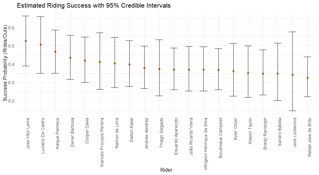
By looking at the 95% confidence intervals we see that there is no rider that is significantly different from the other. Meaning that there isn’t a rider that is significantly better or worse at staying on the bull, if more there was another rodeo the rankings could easily change. The riders with wider intervals have less data so there is more uncertainty. If we added data from other seasons we could really dial in on what the percentages are and get more insight into if riders are really different from one another.

Conclusion

This was a fun project for me to learn about something new and do something a little out of my comfort zone. I would love to do this with other metrics or add in factors like bulls to get more insight in the future.

Back to my original question: how did Rafael José de Brito become the best rider in 2023 despite having low summary metrics? Well, when you look at just one summary stat, it might seem like he’s underperforming. But with a Bayesian approach that accounts for uncertainty and variance, you can see that he holds up just fine against other top riders.

All in all I think it would be really cool to see some more in depth data on bull riding. I love doing these little projects but the hardest part is always finding cool data…so maybe I’ll just have to go in person to a rodeo this summer and collect my own data ;)